A Garden Variety of Bloom Filters

In this article, I explain how Bloom filters work and introduce several variants that evolved as a result of extensive academic treatment of this topic. Moreover, I present libbf, an implementation of these Bloom filters as a C++11 library.

Whenever you have a set or list, and space is an issue, a Bloom filter may be a useful alternative.
–Mitzenmacher

Introduction

A Bloom filter is a randomized synopsis data structure that supports set membership queries. Its space-efficient representation comes at the cost of false positives, i.e., elements can erroneously be reported as members of the set. In practice, the huge space savings often outweigh the false positives if kept at a sufficiently low rate.

Bloom filters have received a great deal of attention not only by the research community but also in practice. For example, Google Chrome uses a Bloom filter to represent a blacklist of dangerous URLs. Each time a user is about to navigate to new page, the corresponding URL is mangled, hashed, and then compared to a local Bloom filter that represents the set of all malicious URLs. If the Bloom filter reports that the URL is in the set, the browser performs a candidate check by sending the hash of the URL to the Safebrowsing server to confirm that the URL is indeed malicious. That is, all checks are performed locally, but when the user surfs to a malicious URL, an extra round trip to the Safebrowsing server occurs.

Another example is the squid web proxy which uses Bloom filters to represent cache digests, which caching servers use to periodically exchange the objects they contain. There are many more examples of Bloom filter applications, for instance in peer-to-peer applications, routing protocols, IP traceback, resource location, etc. Broder and Mitzenmacher give a good survey of network applications.

Bloom Filters

Before we delve into the discussion, let us agree on some common notation.

Terminology

• Universe $U$
• $N$ distinct items
• $k$ independent hash functions $h_1,\dots,h_k$
• Vector $V$ of $m$ cells, i.e., $m = \lvert V \rvert$
• Set:
  • $S = \{x_1,\dots,x_n\}$ where $x_i\in U$ and $\lvert S\rvert = n$
• Multiset / Stream:
  • $\mathcal{S} = \{x_1,\dots,x_n\}$ where $x_i\in U$ and $|\mathcal{S}| = n$
  • $C_x = \left\{ c_{h_1(x)},\dots,c_{h_k(x)} \right\}$ counters of $x$
  • $f_x =$ multiplicity (frequency) of $x\in\mathcal{S}$
• Bloom filter estimate denoted by hat: $\widehat{S}, \widehat{\mathcal{S}}, \widehat{f}_x, \ldots$
• Probability of a false positive (FP): $\phi_P = \mathbb{P}\left(x\in \widehat{S} \vert x\notin S\right)$
• Probability of a false negative (FN): $\phi_N = \mathbb{P}\left(x\notin \widehat{S} \vert x\in S\right)$
• Capacity $\kappa$, i.e., is the maximum number of items a Bloom filter can hold until a given $\phi_P$ can no longer be guaranteed
• A Bloom filter is full when then number of added items exceeds $\kappa$

Basic

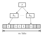Burton Bloom introduced the original Bloom filter in 1970, which I refer to as the basic Bloom filter from now on. The underlying data structure is a bit vector $V$ with $|V| = m = O(n)$ and $k$ independent hash functions $h_1, \dots, h_k$ that map items in $U$ to the range $[m] = \{1,\ldots,m\}$. (Unlike in the implementation, I start at index 1 for the formal treatment.) All bits in $V$ are initialized to 0. Inserting an item $x\in S$ involves setting the bits at positions $h_1(x), \ldots, h_k(x)$ in $V$ to 1. Testing whether an item $q\in U$ is a member of $\widehat{S}$ involves examining the bits at positions $h_1(q),\dots,h_k(q)$ in $V$. If any of these bits is 0 the Bloom filter reports $q\notin \widehat{S}$, and $q\in \widehat{S}$ otherwise. However, there remains some probability that $q\notin S$. This type of error is a false positive (FP) and also known as Bloom error $E_B$. It occurs because other elements in $S$ also map to the same positions.

To compute the probability of a Bloom error, we start off with an empty bit vector $V$ and insert an item. This is the same as independently (and uniformly) choosing $k$ bits and setting them to 1. Thereafter, the probability that a certain bit in $V$ is still 0 is

$$\left(1 - \frac{1}{m}\right)^k.$$

Afer $n$ insertions, the probability that a certain bit is 1 is

$$1 - \left(1 - \frac{1}{m}\right)^{kn}.$$

Testing for membership involves hashing an item $k$ times. Thus the probability of a Bloom error is

$$\begin{equation} \mathbb{P}(E_B) = \left(1-\left(1-\frac{1}{m}\right)^{kn}\right)^k \approx \left(1 - e^{-kn/m}\right)^k \end{equation}$$

For fixed parameters $m$ and $n$, the optimal value $k^*$ that minimizes this probability is

$$k^* = \arg\min_k\;\mathbb{P}(E_B) = \left\lfloor\frac{m}{n}\ln 2\right\rfloor$$

For $k^*$, we have hence $E_B = (0.619)^{m/n}$. Moreover, for a desired FP probability $\phi_P$ we can compute the number of required bits by substituting the optimal value of $k$:

$$m = -\frac{n\ln p}{(\ln 2)^2}.$$

Multisets

A basic Bloom filter can only represent a set, but neither allows for querying the multiplicities of an item, nor does it support deleting entries. I use the term counting Bloom filter to refer to variants of Bloom filters that represent multisets rather than sets. Technically, a counting Bloom filter extends a basic Bloom filter with width parameter $w$. (Note that the original counting Bloom filter used cells with $w=4$ only to support deletion, not to count elements.)

Counting

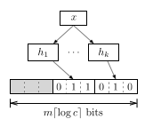In a counting Bloom filter, inserting an item corresponds to incrementing a counter. Some variants also feature a decrement operation to remove item from a set. But deletions necessarily introduce false negative (FN) errors. Think about it this way: when you flip a set bit back to 0 that was part of a $k$ bits from another item, the Bloom filter will no longer report $x\in\widehat{S}$. The probability of a FN is bounded by $O(E_B)$.

Retrieving the count of an item $x\in\widehat{S}$ involves computing its set of counters $C_x$ and returning the minimum value as frequency estimate $\widehat{s}_x$. This query algorithm is also known as minimum selction (MS).

There exist two main issues with counting Bloom filters:

1. Counter overflows
2. The choice of $w$

The first problem exists when the counter value reaches $2^w - 1$ and cannot be incremented anymore. In this case, one typically stops counting as opposed to overflowing and restarting at 0. However, this strategy introduces undercounts, which we also refer to as FNs.

The second problem concerns the choice of the width parameter $w$. A large $w$ quickly diminishes the space savings from using of a Bloom filter. There will also be a lot of unused space manifesting as unused zeros. A small $w$ may quickly lead to maximum counter values. As such, choosing the right value is a difficult trade-off that depends on the distribution of the data.

Bitwise

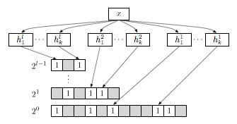The bitwise Bloom filter is a combination of $l$ counting Bloom filters with bit vectors $V_i$, each of which have $m_i$ cells, $k_i$ hash functions, and width $w_i$ where $i\in\{0,\dots,l-1\}$. This variant aims at solving both of the overflow and space problem of the counting Bloom filter.

To add an item $x$, first look at the counters in the first level $V_0$. If there is enough room (i.e., width) available, perform the increment. If the counter overflows, insert $x$ into $V_1$ and remove it from $V_0$. In this fashion, the counter value is conceptually unbounded by adding more and more levels. However, the item has to be hashed $l$ times with a total of $\sum_{i=0}^{l-1} k_i$ hash functions.

Retrieving the counter of an item involves combining the binary representation of all levels. Let $c_i$ be the counter value at level $i$. Then we compute the counter value as

$$C = \sum_{i=0}^{l-1} c_i 2^{\sum_{j=0}^i w_i}.$$

Spectral

The spectral Bloom filter is an optimized version of the counting Bloom filter. It consists of two extra algorithms in addition to MS and introduces a more space-efficient data structure to represent counters.

1. Let us review the MS algorithm. When querying an item $q\in U$, MS uses the minimum counter value $m_q = \min_i\;C_q$ as frequency estimate, i.e., $\widehat{f}_q = m_q$. Cohen and Matias claim that $f_x \le m_x$ and $\mathbb{P}(\widehat{f}_x \neq m_x) = \mathbb{P}(E_B)$ for all $x\in S$.

2. The second spectral algorithm is an optimization for the add operation. When adding an item $x$ to the Bloom filter, the minimum increase (MI) algorithm only increments the minimum counter value(s) $\tilde{C}_x = \min_i\;C_x$. The rationale behind this is that $m_x$ is always the most accurate count, thus MI results in the fewest possible increment operations.

   Because not all counters are incremented on inserts, the effect of deletes is significantly worse and the number of FNs becomes unbounded. Thus, the MI algorithm should not be used when removing of items from a Bloom filter. Cohen and Matias claim that $E_B^{MI} = O(E_B)$ and that if $x$ is drawn uniformly from $U$, then $E_B^{MI} = E_B/k$.

3. The third algorithm is recurring minimum (RM) and involves two Bloom filters, $V_1$ and $V_2$. The key insight behind RM is that items that experience Bloom errors are less likely to have recurring minima counter values. Cohen and Matias found empirically that this applies to approximately 20% of the items. Such items with a unique minimum are maintained in the second Bloom filter to reduce the discrepancy between $f_x$ and $\widehat{f}_x$.

   To query an item $q\in U$ according to the RM algorithm, we look first into the first Bloom filter and check if $q$ has a recurring minimum. If so, we return the minimum counter value. Otherwise we look the minimum counter value from the second Bloom filter, unless it is 0. If it is 0 (i.e., does not exist), we return the minimum counter from the first Bloom filter.

   Since all the items are inserted into the first bloom filter, the RM optimization does at least as well as the MS algorithm, yet has usually better error rates because a second filter holding fewer items is used for items which experience higher error rates.

The fancy data-structure takes $N + o(N) + O(n)$ space, where $n$ is the number of distinct items and $N = k\sum_{x\in S} \lceil \log f_x \rceil$. For details, please refer to the paper.

As an aside: a spectral Bloom filter with MS policy is conceptually isomorphic to the Count-Min Sketch (CMS) when we partition the underlying bit vector into $k$ sections, with each $h_i$ mapping to section $i$. Similarly, we can derive the Fast-AMS sketch by taking the median of the $k$ counters instead of their minimum.

Aging

A problem all the above Bloom filter variants is that they eventually fill up over time when dealing with a large set or stream of data. This means that at some point the Bloom filter becomes unusable due to its high error rates. There exist various scenarios where one would like to “age out” old items that have been added a long time ago. For example, we might want to estimate only recent items or we have a very limited amount of space available.

Although counting Bloom filters have a delete operation, it is often impossible to retain old items in memory. Thus we do not know their counter positions in the bit vector anymore, otherwise we would simply decrement their count. What we want is a Bloom filter that has sliding window semantics, as illustrated by the Figure below.

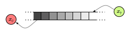
To support a sliding window, we would like a Bloom filter which acts like a FIFO. In the following, I discuss two different Bloom filter flavors that aim at providing this property.

Stable

The stable Bloom filter is essentially a basic Bloom filter with an underlying bit vector with a fixed cell width $w$. However, counters do not represent the multiplicities of the items but rather their age. Thus the interface supports only set membership queries.

To insert an item, we decrement $d$ cells chosen uniformly at random. Thereafter, we set the counters of all $k$ cells to their maximum value of $2^w - 1$.

Deng and Rafiei have shown that the fraction of zeros will eventually become constant. When having reached this stable point, the approximate probability of a Bloom error is

$$\phi_P \approx 1 - \frac{1}{1+\frac{1}{d(1/k-1/m)}} = \frac{1}{d/k-d/m+1}$$

A²

The $A^2$ Bloom filter, also known as active-active buffering, provides another type of FIFO. It uses two single-bit vectors $V_1$ and $V_2$ where $|V_1| = |V_2| = \frac{m}{2}$. Unlike the spectral RM algorithm, one Bloom filter is not a subset of the other, so an item can be in either Bloom filter.

The algorithm works as follows. To query for an item, return true if $q$ exists in either $V_1$ or $V_2$. To insert an item $x$, simply return if it already exists in $V_1$. Otherwise insert it in $V_1$ and test whether $V_1$ has reached its capacity. If it is full, flush $V_2$ and swap $V_1$ and $V_2$. Thereafter insert the item in $V_1$ (the old $V_2$).

One advantage of the $A^2$ Bloom filter is space-efficiency, since one bit vector is always full. Let the subscript $a$ denote the value of the $A^2$ Bloom filter. The probability of a Bloom error is

$${\phi_P}_a = 1 - \sqrt{1-\phi_P}$$

and the optimal value for $k_a$ and $\kappa_a$ are:

$$k_a^* = \left\lfloor -\log_2\left(1-\sqrt{1-\phi_P}\right) \right\rfloor \qquad \kappa_a^* = \left\lfloor \frac{m}{2k_a^*} \ln2 \right\rfloor$$

libbf

As part of a class project for the course Combinatorial Algorithms and Data Structures in Spring 2011 at UC Berkeley, I decided to write a C++11 library of Bloom filters, libbf, which implements the above discussed Bloom filters. Slides of the final presentation are also available; they go a little deeper into the algorithmic details. Note that the slides cover an early version of the implementation; the API has changed significantly since.

Related Work

I only presented a few Bloom filter types in this article, but active research in this field yielded many more variations. For example, the dynamic and scalable Bloom filter are two variants that grow dynamically as soon as more items are added. Bloom filters can also be compressed, e.g., when sending them over the network. Distance-sensitive Bloom filters give more than a binary answer or count when asking for an item: they also return if an item is close to another item in the set. Finally, there exist Bloomier filters which extend the set membership query model and counting notion to computations of arbitrary functions.

Cuckoo hashing is a related space-efficient alternative to Bloom filters. Moreover, Adam Langley has some interesting thoughts on Golomb Compressed Sets. Finally, Ilya’s article on probabilistic data structures for data mining presents a nice follow-up read.

Acknowledgements

I would like to thank Ryan Killea and Tobin Baker for their useful feedback.

Load Comments